
The Big Picture is the name of Barry Ritholtz’s blog about stocks, investing, financial markets, and economics. Interestingly, I actually ran across this good blog will searching for Godel, Escher, Bach.
Category: stocks (Page 4 of 6)
The works of Didier Sornette and others show that Log-Periodic Power Law (LPPL) oscillations occur before financial crashes. Implementing the ideas found in various papers, the following graphs were created. As can be seen from the following graphs, peaks in the periodogram signals occurs shortly before some of the crashes.
I created a blog devoted to exploring these LPPL market signals: LPPL Market Watch
Update: new website devoted to this subject. Visit: The Bubble Index.
Summary of Research
Recent research by Didier Sornette and his colleagues suggests that market crashes are predictable phenomenon. Even though economists debate the existence of crashes and their precursors – bubbles, there exists historical proof of Log-Periodic Power Law (LPPL) oscillations occurring immediately before all recorded major market declines in all major stock indices. For example, these LPPL oscillations occurred in the Dow Jones Industrial Average and S&P 500 shortly before the crashes of 1929, 1987, and 2000.
With the aide of Sornette’s previous papers on market crashes, a “bubble index” is created. The bubble index displays the likelihood of a market bubble at any given time. With an index like this as a tool, any investment strategy which seeks to time the market will be highly successful. The bubble index indicates when to change asset positions in preparation for an incoming crash. One application of the bubble index is for financial planners and investment managers to change their client’s asset allocations accordingly. As the bubble index spikes, a crash is near. After the crash occurs the bubble index returns to low levels, indicating that the crash is over.
A bubble index for both the Dow Jones Industrial Average and the S&P 500 is formed with the methods presented in this paper. Remarkably, the 1929, 1962, 1987, and 2000 crashes are all predicted at least a week before the actual crash. In the weeks prior to these crashes there is a large spike in the index. After the crash occurs, the index returns to low levels. Interestingly, the bubble index for these indices only spikes during a crash. In other words, given that a spike has occurred, there is a 100% probability that a crash has or will occur. However, some of the crashes are not predicted by spikes in the bubble index. For instance, In both indices the 1968, 1972, and the 2008 crash show no spike in the index before or during the event.
These LPPL signals indicate that crashes are not related to changes in technology, culture, economic policies, etc… In other words, financial markets have patterns which suggest an underlying structural instability during crashes. This supports Sornette’s belief that financial crashes are critical phenomena resulting from the complex interactions of traders. To me, this suggests that the natural sciences have a key place in finance.
The implications of these results are rather enormous, since the index is simple to create and understand. The ability to leave the market before a crash and enter after the event provides a wonderful opportunity to earn excess returns while preserving capital. This bubble index should be run on a daily basis to allow an investment manager or financial planner to gain an awareness of current stability conditions. If the bubble index is widely viewed and accepted as a legitimate and reliable forecast of bubbles and crashes, then crash prevention may be possible at the macro level.
Links to papers:
May 16, 2013 – Update:
 |
| Figure 1 |
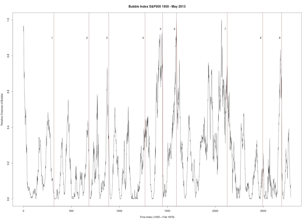
Figure 1 produced with C++ code. S&P 500. Seven year window of data. Every data point is a new week (vs. other graphs where every data point is a change of 4 weeks). Every peak in the market is corresponded by vertical line.
1. January 17, 1966 — followed by a 20.9% drop
2. January 15, 1973 — followed by a drop in excess of 23%
3. December 27, 1976 — followed by a drop in excess of 14.7%
4. March 26, 1984 — followed by a 11.8% drop
5. Sept. 28, 1987 — followed by a 31.7% drop
6. July 9, 1990 — followed by a 17.4% drop
7. August 28, 2000 — followed by a 36.5% drop
8. October 1, 2007 — followed by a drop in excess of 42%
9. July 18, 2011 — followed by a 16.5% drop
 |
| Figure 2 |
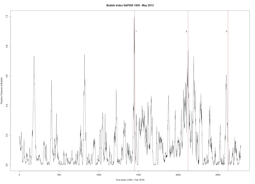
Figure 2 was produced with C++ code. S&P 500. Six year window of data.
1. Sept. 28, 1987 — followed by a 31.7% drop
2. August 28, 2000 — followed by a 36.5% drop
3. April 19, 2010 — followed by a 16% drop
 |
| Figure 3 |
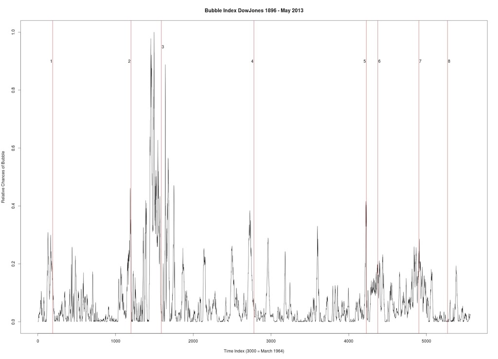
Figure 3 was produced with C++ code. Dow Jones Industrial Average. Six year window of data.
1. December 31, 1909 — followed by a 23% drop
2. October 2, 1929 — followed by a 43% drop
3. March 12, 1937 — followed by a 40% drop
4. January 8, 1960 — followed by a 15.6% drop
5. October 2, 1987 — followed by a 31.7% drop
6. July 27, 1990 — followed by a 17% drop
7. September 8, 2000 — followed by a 36% drop
8. October 12, 2007 — followed by a drop in excess of 42%
 |
| Figure 4 |
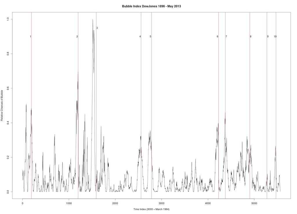
Figure 4 was produced with C++ code. Dow Jones Industrial Average. Seven year window of data.
1. December 31, 1909 — followed by a 23% drop
2. October 2, 1929 — followed by a 43% drop
3. March 12, 1937 — followed by a 40% drop
4. September 23, 1955 — followed by a quick 8.7% drop and then recovery
5. January 8, 1960 — followed by a 15.6% drop
6. October 2, 1987 — followed by a 31.7% drop
7. July 27, 1990 — followed by a 17% drop
8. September 8, 2000 — followed by a 36% drop
9. October 12, 2007 — followed by a drop in excess of 42%
10. July 8, 2011 — followed by a 16% drop
Modelling market returns as independent random variables/martingales is the same as modelling the solar system as a geocentric system with the planets and Sun circling around Earth in epicycles. Predictions of the future are often vastly incorrect in both models. Quite surprisingly, this solar system model survived for thousands of years, despite it being totally incorrect. Then came Tycho Brahe who introduced a modified version of this Ptolemaic system. In Brahe’s model the planets orbit the Sun which orbits the Earth. While this model improved the accuracy of planetary motions, it failed to model reality. Perhaps it could be said that stochastic jump processes are equivalent to Brahe’s model of the solar system. While these jump process do a better job at modelling the returns than simple stochastic processes, they fail to grasp the underlying true model of returns.
 |
| Poor Market Forecasting |
And as we now know, the true model (for now) of the solar system was introduced by Aristarchus (Copernicus and Kepler helped bring forward this model) and predicts planetary motions with near perfection and represents the actual state of the solar system. I believe that the analogous model for stock returns has been introduced by Didier Sornette, Anders Johanson and others.
These scientists have expounded the idea that market returns are a function of individual agents in a complex system. Just as the human body is a collection of individual cells which make “decisions” based on communications with neighbours through chemical processes, traders make their own decisions based on communication with neighbours. With this perspective the market is a complex system of interacting agents. Thus, returns should be a function of these interactions. Under this complex system model, bubbles and crashes which dot the history of finance (which are not explained fully by independent returns/martingales) are straightforward results. In addition, these models still explain why returns are close to normal “most” of the time.
So, it seems that we need to modify or throw away the old models in favour of these new complex system models. These complex models offer better prediction of the overall market and more fully represent reality.
There is the interesting possibility of this: the stochastic volatility model referred to as the Ornstein-Uhlenbeck process represents the physical process of a “noisy relaxation process.” The Wiener Process represents Brownian motion or motion of a particle through a gas or liquid. So, if we consider the movement of a stock through a virtual container of many stocks (these stocks are the atoms in the Brownian motion) then we need to ask ourselves: What does the price, interest rate, returns, etc. mimic? It is NOT the equations! BUT the physical processes themselves. Why is an interest rate in a state of disequilibrium in the first place… that it must try to relax? Who put the stock in swarm of human hands all independently moving… It more correctly seems that the traders are following its movement at every second, waiting to grab it when the time if right (thus not independent)?
Zero Hedge is veritable gold mine of website links and good articles on economics, finance, and markets. Its mission statement:
- to widen the scope of financial, economic and political information available to the professional investing public.
- to skeptically examine and, where necessary, attack the flaccid institution that financial journalism has become.
- to liberate oppressed knowledge.
- to provide analysis uninhibited by political constraint.
- to facilitate information’s unending quest for freedom.
Let’s say that you have started an IRA or some sort of long term retirement account. One strategy would be to invest 100% of your money in an index fund which follows the S&P 500. This would give you around 9 – 11% annual average returns over 50+ years. However, you will notice that there are several times throughout the life of the account in which the index suffers massive losses.
To counteract these loses it would be wise to find another index, such as a short term bond fund, where you could temporarily store your returns; then, once the market has crashed, you could invest these funds back into the stock market.
This strategy is a modified version of the one suggested by Benjamin Graham in The Intelligent Investor. His strategy was to always be in a range of 25-75% in a bond and stock fund. In other words, never have your portfolio more than 75% or less than 25% in either bonds or stocks. Then, depending on whether you “felt” the market was too optimistic or too pessimistic you would adjust your ratios accordingly. I feel that this idea of optimism and pessimism can somehow be quantified and developed into an algorithm.
Take two index funds: the S&P 500 index fund and a two year bond fund. Both have minimal expenses (Vanguard funds). The strategy is simple. Begin with 70% in stocks and 30% in bonds and wait 24 months. Now, check the past 24 months. Is there a gain or loss of magnitude greater than 50% in the S&P 500 index during this period? If true, then readjust your portfolio. If it is a gain, then bring the portfolio back to 70% S&P 500 index and 30% bond fund. If it is a loss, then bring the portfolio to 95% S&P 500 and 5% bond fund. Repeat this process every 24 months. Also, make sure you continue to make monthly deposits 50-50 into the stock and bond funds.
Performing this strategy with certain adjustments in these ratios will allow the investor to achieve better than market annual average returns for 50+ years. I am currently trying to work out the exact results and best parameters of this strategy. I believe these returns will be even better depending on the amount invested per month.
Sadly, most people make the mistake of decreasing their stock holdings right after a crash and increasing their stock holdings during a bull market which precedes a crash. This psychological reflex will lower the net return drastically.

