Stock prices, as seen by many appear to be purely random processes with no patterns and thus no predictability. And more often than not, people unfamiliar with stochastic processes will equate the work of financial engineers as “hocus-pocus,” “rocket science,” or just plan gambling. Are these people correct? Are asset managers playing roulette with the public’s money? If so, then it would seem that the life work of people such as Ito, Merton, Black, Scholes, Hull, Cox, White, Detemple, Sornette, and others amount to no more than speculation or the ramblings of an inmate in an insane asylum. Assuming otherwise, and that there is method to the madness of these academics, prices are predictable. And stochastic calculus provides a framework with which to build predictions. But how well and how reliable are the calculations? How can we use this predictability to properly manage risk?
There are at least two important responsibilities for risk managers:
1. Risk managers must make rational decisions. An empirical and purely quantitative forecast of future returns should be made with a clear understand of model assumptions.
2. With the foresight provided by the model, a suitable strategy must be taken. If the observations are indicating current market bubble conditions, then managers should be selling, or at the very least not buying.
These responsibilities are general and do not depend on the model being implemented to forecast returns. The accuracy of the forecast depends greatly on the assumptions used to create the model. The majority of models assume:
1. That returns are independent in time.
2. That volatility is constant.
3. That markets are efficient.
4. That prices follow the Geometric Brownian Motion
In other words, most models assume that human emotions, psychology, and behavior are not factors in determining the price movements of assets. How can such critical factors be ignored by financial engineers? The number of papers dealing with the effects of behavior on stochastic equations are few. Instead, the academic community has and continues to brush off these factors with the wrongly conceptualized idea that the sum total of all human interactions will create Brownian Motion. The billions of collisions on a grain of pollen in H2O are what stirred the creation of this type of stochastic process. So, the question is: Can we equate the process which creates Browian Motion as observed by Brown himself, to the structure of asset price movement? One is created through thermal random thermal interactions; the other through human emotion, psychology, and behaviour.
Risk managers should realize these assumptions and they should be cautious.
If risk managers believe in the predicatablity of prices, then we must, by force of principle assume that there is an underlying structure. In other words, consider the prediction of Earthquakes. The fact that we even consider the ability to predict their occurrence suggests that we have some degree of knowledge regarding their underlying structure. By believing in the predictability of price trajectories, we naturally assume some underlying structure. But what is this structure? How do we monitor the processes at work?
Are returns predictable? According to much research, the answer to this question is a firm, yes. But arbitrage theory says that such predicatablity can not exist. So, what does the risk manager believe? Does he believe that prices are Brownian Motions; that markets are efficient machines, not affected by the emotions, psychology, and behavior of humans; or does he disregard these assumptions in search for a better stochastic model? The answer to this question lies in controversy and may not be resolved for a long time. However, the risk manager has 100 billion of assets which he must manage today. Where is he to look for alternative models which disregard the assumptions of his collegues and predecessors? This paper provides the beginning of one such alternative.
This paper presents a stochastic model of the form: change(price) = function(volume). The volume depends on a matrix with a fixed number of agents. The intuition behind this model comes from the concept that a stock price’s movement should reflect not a normal distribution, which has roots in the idea of Brownian motion and particles in heat transfer, but rather a bi-directional “tug-of-war” between agents who are buying and selling with human emotions, psychology, and behavior. Just as in the youthful tug-of-war game, there are times when it appears that the right side has the upper hand, when, all of the sudden the left side makes a determined effort and brings down the right side. These drastic and rapid phase transitions are unheard of in a Brownian idea of price movements. The Brownian application to asset price movements provide a decent first approximation. However, stochastic processes with Brownian Motion will never evolve in a manner to explain the stylized facts observed from the actual distribution of asset returns. Thus, to truly model price behavior, practitioners should study the fundamental structure of the market.
Consider this thought experiment:
Take a snapshot of all market participants in a security XYZ. This is period zero (t = 0). Suppose there are a fixed number, N, total people in the financial system who can own and trade XYZ. In other words, the price movement of this asset should depend only on the actions of these N traders. Now count the number of traders who currently hold a short position in XYZ and a long position in XYZ. Let S0and L0 represent the number of traders who are currently short and long, respectively, the asset XYZ. Let S0 + L0< N, thus there are a number of traders, H0, who hold neither a short nor a long position. Thus, H0 = N – S0– L0. The current price of XYZ is P0. Assume that all transactions only involve 1 share of XYZ. Further posts will seek to address the important consideration of number of shares.
Now consider the next possible moves for all traders in the market (t = 1). There are assumed to be four possibilities:
- An XYZ owner with a long position sells. (L1 = L0 – 1 and H1 = H0+ 1)
- A trader short XYZ covers his/her position. (S1 = S0 – 1 and H1 = H0+ 1)
- A neutral trader initiates a long position. (L1 = L0 + 1 and H1 = H0– 1)
- A neutral trader initiates a short position. (S1 = S0 + 1 and H1 = H0 – 1)
Thus, numbers 1 and 2 increase the number of neutral traders, while 3 and 4 decrease that number. Assume that both 2 and 3 cause the price of XYZ to increase by some factor and 1 and 4 decrease the price of XYZ by the same factor. Thus the movement of the price of XYZ should be a bi-directional “tug-of-war” battle: traders going long and shorts covering versus traders shorting and longs selling.
To represent this computationally, a matrix can be created which holds the current state of all traders. To create the initial state matrix, called StateMatrix0, form an √N x √N square matrix (for simplification, it would be best to choose N as a perfect square). Then fill the matrix randomly with the value -1 for the correct number of traders short XYZ, S0. Do likewise with L0and H0, represented by 1 and 0, respectively. Thus, the initial StateMatrix0 will be randomly filled with {-1,0,1}, representing the traders who are short, neutral, and long.
Now, proceed one period to t = 1. To calculate the next StateMatix1, do the following:
Assume that each trader is influenced by U of his peers and that this influence is proportional to a factor representing the general market “mood.” Call the mood factor for the current period, Mt. To find what the trader will do in the transition from t = 0 to t =1, sum the values of his U neighbors, find their average, multiply by the current Mt and round. In addition, include a possibility for trader[i,j] to form his own independent value {-1,0,1} and ignore his U neighbors with probability, IDIO (an idiosyncratic change of asset position).
- For example, suppose that at t = 0, trader[i,j] of the matrix was short, i.e. the value was -1 and that his 4 neighbors at i = 0 had values {1,0,1,-1}. Suppose the M1 at this time is 1.2 and IDIO = 0.20. If this trader[i,j] does not choose an idiosyncratic position, then he mimics his neighbors. The sum of his four neighbors is thus SumTrader[i,j] = 1 + 0 + 1 – 1 = 1 and the average is ¼. Thus ¼*1.2 = 0.3. Rounding give a value of 0. Thus, the trader[i,j] should change his value to 0, in other words the trader[i,j] will cover his position.
Performing this calculation for every trader on the grid will create the StateMatrix1. And doing this for T periods will create a StateMatrix{t=[0,T]} sequence of trader states. To calculate the actual price movement based on this model do the following:
- Sum over all values of trader[i,j] of StateMatrixt
- Sum over all values of trader[i,j] of StateMatrixt+1
- Calculate the difference, StateMatrixt+1 – StateMatrixt and divide by N. Multiply by Pt. This value = C, the change in the price from the previous price
- Pricet+1 = Pricet+ C
This will form the evolution of the price through the states of the StateMatrix{t=[0,T]} sequence.
Note: In order to make the Mtfactor suitable, its values must fall between [0,1.5). If not, then values of the traders[i,j] may be other than {-1,0,1}. The Mt factor can be calculated at each period with the following calculation:
In other words, the Mood factor Mtfor the next period is the ratio of the number of current traders who are long to the number of current traders who are short. There may be other ways to define this factor.
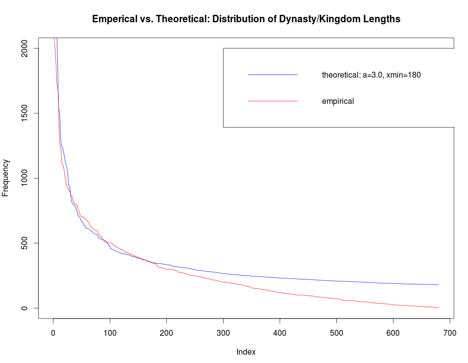
Look at the previous
post, here, to see an example. In that post I used: