The works of Didier Sornette and others show that Log-Periodic Power Law (LPPL) oscillations occur before financial crashes. Implementing the ideas found in various papers, the following graphs were created. As can be seen from the following graphs, peaks in the periodogram signals occurs shortly before some of the crashes.
Summary of Research
Recent research by Didier Sornette and his colleagues suggests that market crashes are predictable phenomenon. Even though economists debate the existence of crashes and their precursors – bubbles, there exists historical proof of Log-Periodic Power Law (LPPL) oscillations occurring immediately before all recorded major market declines in all major stock indices. For example, these LPPL oscillations occurred in the Dow Jones Industrial Average and S&P 500 shortly before the crashes of 1929, 1987, and 2000.
With the aide of Sornette’s previous papers on market crashes, a “bubble index” is created. The bubble index displays the likelihood of a market bubble at any given time. With an index like this as a tool, any investment strategy which seeks to time the market will be highly successful. The bubble index indicates when to change asset positions in preparation for an incoming crash. One application of the bubble index is for financial planners and investment managers to change their client’s asset allocations accordingly. As the bubble index spikes, a crash is near. After the crash occurs the bubble index returns to low levels, indicating that the crash is over.
A bubble index for both the Dow Jones Industrial Average and the S&P 500 is formed with the methods presented in this paper. Remarkably, the 1929, 1962, 1987, and 2000 crashes are all predicted at least a week before the actual crash. In the weeks prior to these crashes there is a large spike in the index. After the crash occurs, the index returns to low levels. Interestingly, the bubble index for these indices only spikes during a crash. In other words, given that a spike has occurred, there is a 100% probability that a crash has or will occur. However, some of the crashes are not predicted by spikes in the bubble index. For instance, In both indices the 1968, 1972, and the 2008 crash show no spike in the index before or during the event.
These LPPL signals indicate that crashes are not related to changes in technology, culture, economic policies, etc… In other words, financial markets have patterns which suggest an underlying structural instability during crashes. This supports Sornette’s belief that financial crashes are critical phenomena resulting from the complex interactions of traders. To me, this suggests that the natural sciences have a key place in finance.
The implications of these results are rather enormous, since the index is simple to create and understand. The ability to leave the market before a crash and enter after the event provides a wonderful opportunity to earn excess returns while preserving capital. This bubble index should be run on a daily basis to allow an investment manager or financial planner to gain an awareness of current stability conditions. If the bubble index is widely viewed and accepted as a legitimate and reliable forecast of bubbles and crashes, then crash prevention may be possible at the macro level.
Links to papers:
May 16, 2013 – Update:
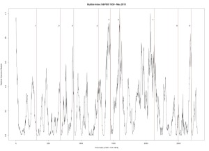 |
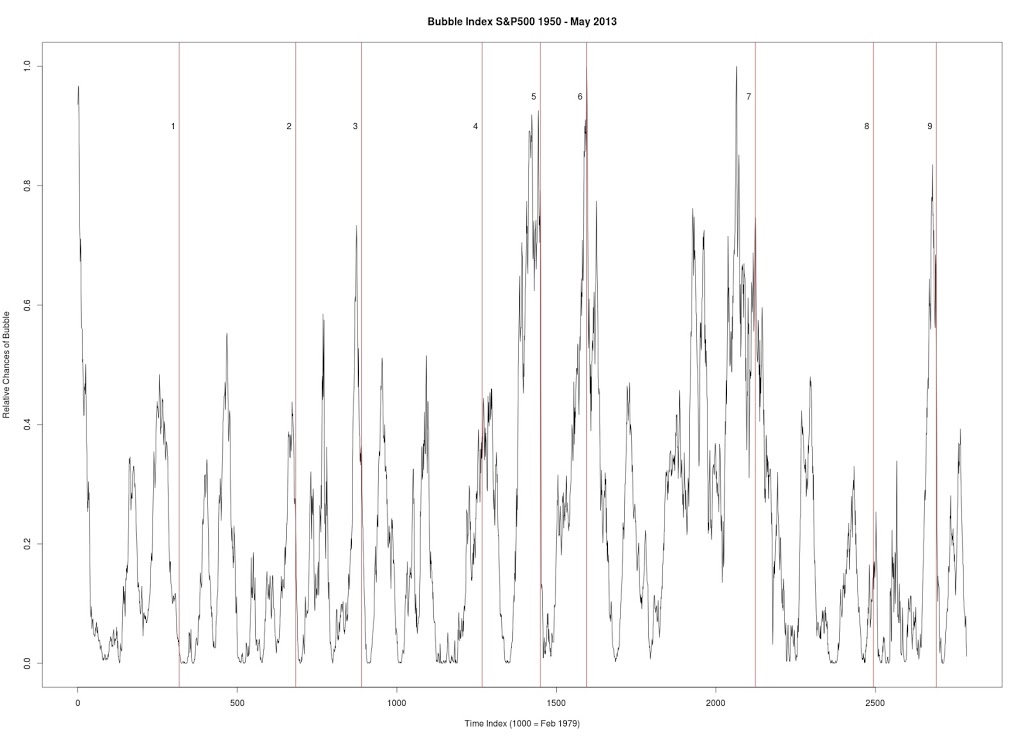
| Figure 1 |
Figure 1 produced with C++ code. S&P 500. Seven year window of data. Every data point is a new week (vs. other graphs where every data point is a change of 4 weeks). Every peak in the market is corresponded by vertical line.
1. January 17, 1966 — followed by a 20.9% drop
2. January 15, 1973 — followed by a drop in excess of 23%
3. December 27, 1976 — followed by a drop in excess of 14.7%
4. March 26, 1984 — followed by a 11.8% drop
5. Sept. 28, 1987 — followed by a 31.7% drop
6. July 9, 1990 — followed by a 17.4% drop
7. August 28, 2000 — followed by a 36.5% drop
8. October 1, 2007 — followed by a drop in excess of 42%
9. July 18, 2011 — followed by a 16.5% drop
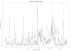 |
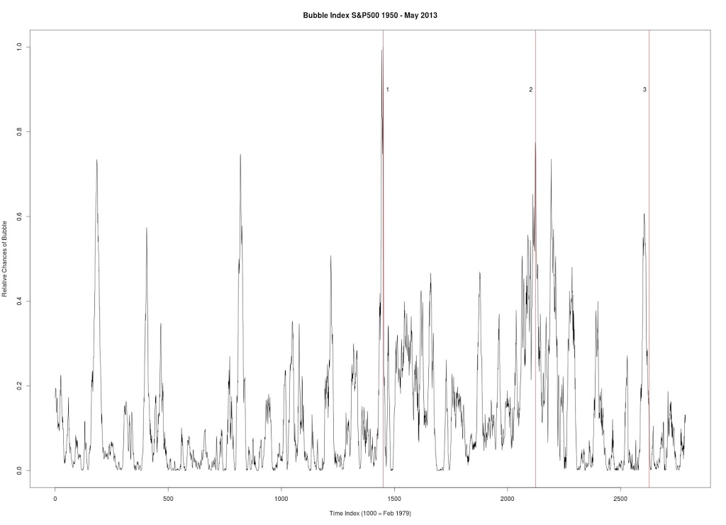
| Figure 2 |
Figure 2 was produced with C++ code. S&P 500. Six year window of data.
1. Sept. 28, 1987 — followed by a 31.7% drop
2. August 28, 2000 — followed by a 36.5% drop
3. April 19, 2010 — followed by a 16% drop
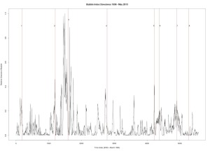 |
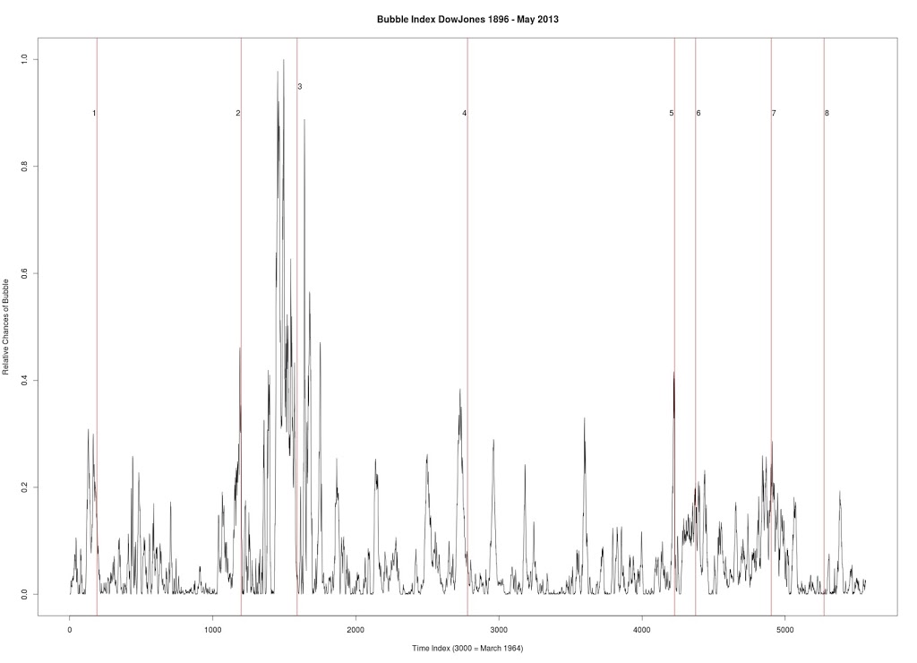
| Figure 3 |
Figure 3 was produced with C++ code. Dow Jones Industrial Average. Six year window of data.
1. December 31, 1909 — followed by a 23% drop
2. October 2, 1929 — followed by a 43% drop
3. March 12, 1937 — followed by a 40% drop
4. January 8, 1960 — followed by a 15.6% drop
5. October 2, 1987 — followed by a 31.7% drop
6. July 27, 1990 — followed by a 17% drop
7. September 8, 2000 — followed by a 36% drop
8. October 12, 2007 — followed by a drop in excess of 42%
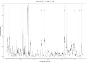 |
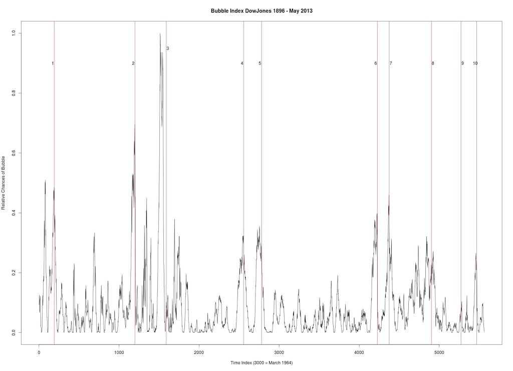
| Figure 4 |
Figure 4 was produced with C++ code. Dow Jones Industrial Average. Seven year window of data.
1. December 31, 1909 — followed by a 23% drop
2. October 2, 1929 — followed by a 43% drop
3. March 12, 1937 — followed by a 40% drop
4. September 23, 1955 — followed by a quick 8.7% drop and then recovery
5. January 8, 1960 — followed by a 15.6% drop
6. October 2, 1987 — followed by a 31.7% drop
7. July 27, 1990 — followed by a 17% drop
8. September 8, 2000 — followed by a 36% drop
9. October 12, 2007 — followed by a drop in excess of 42%
10. July 8, 2011 — followed by a 16% drop