An Autonomous Agent

exploring the noosphere

Category: phase transitions (Page 1 of 2)

Price Simulation of Trader Matrix Video

The following video is the time evolution of a network of 10,000 traders and their effect on the price movement of a stock.

For more information, please read the following paper:

An Interesting Model of Asset Price Behavior using a Tri-Valued Matrix of States

Stock prices, as seen by many appear to be purely random processes with no patterns and thus no predictability. And more often than not, people unfamiliar with stochastic processes will equate the work of financial engineers as “hocus-pocus,” “rocket science,” or just plan gambling. Are these people correct? Are asset managers playing roulette with the public’s money? If so, then it would seem that the life work of people such as Ito, Merton, Black, Scholes, Hull, Cox, White, Detemple, Sornette, and others amount to no more than speculation or the ramblings of an inmate in an insane asylum. Assuming otherwise, and that there is method to the madness of these academics, prices are predictable. And stochastic calculus provides a framework with which to build predictions. But how well and how reliable are the calculations? How can we use this predictability to properly manage risk?
There are at least two important responsibilities for risk managers:
1. Risk managers must make rational decisions. An empirical and purely quantitative forecast of future returns should be made with a clear understand of model assumptions.
2. With the foresight provided by the model, a suitable strategy must be taken. If the observations are indicating current market bubble conditions, then managers should be selling, or at the very least not buying.
These responsibilities are general and do not depend on the model being implemented to forecast returns. The accuracy of the forecast depends greatly on the assumptions used to create the model. The majority of models assume:
1. That returns are independent in time.
2. That volatility is constant.
3. That markets are efficient.
4. That prices follow the Geometric Brownian Motion
In other words, most models assume that human emotions, psychology, and behavior are not factors in determining the price movements of assets. How can such critical factors be ignored by financial engineers? The number of papers dealing with the effects of behavior on stochastic equations are few. Instead, the academic community has and continues to brush off these factors with the wrongly conceptualized idea that the sum total of all human interactions will create Brownian Motion. The billions of collisions on a grain of pollen in H2O are what stirred the creation of this type of stochastic process. So, the question is: Can we equate the process which creates Browian Motion as observed by Brown himself, to the structure of asset price movement? One is created through thermal random thermal interactions; the other through human emotion, psychology, and behaviour.
Risk managers should realize these assumptions and they should be cautious.
If risk managers believe in the predicatablity of prices, then we must, by force of principle assume that there is an underlying structure. In other words, consider the prediction of Earthquakes. The fact that we even consider the ability to predict their occurrence suggests that we have some degree of knowledge regarding their underlying structure. By believing in the predictability of price trajectories, we naturally assume some underlying structure. But what is this structure? How do we monitor the processes at work?
Are returns predictable? According to much research, the answer to this question is a firm, yes. But arbitrage theory says that such predicatablity can not exist. So, what does the risk manager believe? Does he believe that prices are Brownian Motions; that markets are efficient machines, not affected by the emotions, psychology, and behavior of humans; or does he disregard these assumptions in search for a better stochastic model? The answer to this question lies in controversy and may not be resolved for a long time. However, the risk manager has 100 billion of assets which he must manage today. Where is he to look for alternative models which disregard the assumptions of his collegues and predecessors? This paper provides the beginning of one such alternative.
This paper presents a stochastic model of the form: change(price) = function(volume). The volume depends on a matrix with a fixed number of agents. The intuition behind this model comes from the concept that a stock price’s movement should reflect not a normal distribution, which has roots in the idea of Brownian motion and particles in heat transfer, but rather a bi-directional “tug-of-war” between agents who are buying and selling with human emotions, psychology, and behavior. Just as in the youthful tug-of-war game, there are times when it appears that the right side has the upper hand, when, all of the sudden the left side makes a determined effort and brings down the right side. These drastic and rapid phase transitions are unheard of in a Brownian idea of price movements. The Brownian application to asset price movements provide a decent first approximation. However, stochastic processes with Brownian Motion will never evolve in a manner to explain the stylized facts observed from the actual distribution of asset returns. Thus, to truly model price behavior, practitioners should study the fundamental structure of the market.
Consider this thought experiment: 
Take a snapshot of all market participants in a security XYZ. This is period zero (t = 0). Suppose there are a fixed number, N, total people in the financial system who can own and trade XYZ. In other words, the price movement of this asset should depend only on the actions of these N traders. Now count the number of traders who currently hold a short position in XYZ and a long position in XYZ. Let S0and L0 represent the number of traders who are currently short and long, respectively, the asset XYZ. Let S0 + L0< N, thus there are a number of traders, H0, who hold neither a short nor a long position. Thus, H0 = N – S0– L0. The current price of XYZ is P0. Assume that all transactions only involve 1 share of XYZ. Further posts will seek to address the important consideration of number of shares.
Now consider the next possible moves for all traders in the market (t = 1). There are assumed to be four possibilities:
  1. An XYZ owner with a long position sells. (L1 = L0 – 1 and H1 = H0+ 1)
  2. A trader short XYZ covers his/her position. (S1 = S0 – 1 and H1 = H0+ 1)
  3. A neutral trader initiates a long position. (L1 = L0 + 1 and H1 = H0– 1)
  4. A neutral trader initiates a short position. (S1 = S0 + 1 and H1 = H0 – 1)
Thus, numbers 1 and 2 increase the number of neutral traders, while 3 and 4 decrease that number. Assume that both 2 and 3 cause the price of XYZ to increase by some factor and 1 and 4 decrease the price of XYZ by the same factor. Thus the movement of the price of XYZ should be a bi-directional “tug-of-war” battle: traders going long and shorts covering versus traders shorting and longs selling. 
To represent this computationally, a matrix can be created which holds the current state of all traders. To create the initial state matrix, called StateMatrix0, form an N x N square matrix (for simplification, it would be best to choose N as a perfect square). Then fill the matrix randomly with the value -1 for the correct number of traders short XYZ, S0. Do likewise with L0and H0, represented by 1 and 0, respectively. Thus, the initial StateMatrix0 will be randomly filled with {-1,0,1}, representing the traders who are short, neutral, and long.
Now, proceed one period to t = 1. To calculate the next StateMatix1, do the following:
Assume that each trader is influenced by U of his peers and that this influence is proportional to a factor representing the general market “mood.” Call the mood factor for the current period, Mt. To find what the trader will do in the transition from t = 0 to t =1, sum the values of his U neighbors, find their average, multiply by the current Mt and round. In addition, include a possibility for trader[i,j] to form his own independent value {-1,0,1} and ignore his U neighbors with probability, IDIO (an idiosyncratic change of asset position).
  1. For example, suppose that at t = 0, trader[i,j] of the matrix was short, i.e. the value was -1 and that his 4 neighbors at i = 0 had values {1,0,1,-1}. Suppose the M1 at this time is 1.2 and IDIO = 0.20. If this trader[i,j] does not choose an idiosyncratic position, then he mimics his neighbors. The sum of his four neighbors is thus SumTrader[i,j] = 1 + 0 + 1 – 1 = 1 and the average is ¼. Thus ¼*1.2 = 0.3. Rounding give a value of 0. Thus, the trader[i,j] should change his value to 0, in other words the trader[i,j] will cover his position.
Performing this calculation for every trader on the grid will create the StateMatrix1. And doing this for T periods will create a StateMatrix{t=[0,T]} sequence of trader states. To calculate the actual price movement based on this model do the following:
  1. Sum over all values of trader[i,j] of StateMatrixt
  2. Sum over all values of trader[i,j] of StateMatrixt+1
  3. Calculate the difference, StateMatrixt+1 – StateMatrixand divide by N. Multiply by Pt. This value = C, the change in the price from the previous price
  4. Pricet+1 = Pricet+ C
This will form the evolution of the price through the states of the StateMatrix{t=[0,T]} sequence.
Note: In order to make the Mtfactor suitable, its values must fall between [0,1.5). If not, then values of the traders[i,j] may be other than {-1,0,1}. The Mt factor can be calculated at each period with the following calculation:
Mt = #Lt-1/#St-1
In other words, the Mood factor Mtfor the next period is the ratio of the number of current traders who are long to the number of current traders who are short. There may be other ways to define this factor.
Look at the previous post, here, to see an example. In that post I used:
N = 1,000,000
T = 700
U = 4
S0 = 0.4*N 
L0 = 0.4*N
IDIO = 0.19

Log-Periodic Power Law Oscillations (LPPL) to Predict Market Crashes

The works of Didier Sornette and others show that Log-Periodic Power Law (LPPL) oscillations occur before financial crashes. Implementing the ideas found in various papers, the following graphs were created. As can be seen from the following graphs, peaks in the periodogram signals occurs shortly before some of the crashes. 
I created a blog devoted to exploring these LPPL market signals: LPPL Market Watch
Update: new website devoted to this subject. Visit: The Bubble Index.
Summary of Research
Recent research by Didier Sornette and his colleagues suggests that market crashes are predictable phenomenon. Even though economists debate the existence of crashes and their precursors – bubbles,  there exists historical proof of Log-Periodic Power Law (LPPL) oscillations occurring immediately before all recorded major market declines in all major stock indices. For example, these LPPL oscillations occurred in the Dow Jones Industrial Average and S&P 500 shortly before the crashes of 1929, 1987, and 2000.
With the aide of Sornette’s previous papers on market crashes, a “bubble index” is created. The bubble index displays the likelihood of a market bubble at any given time. With an index like this as a tool, any investment strategy which seeks to time the market will be highly successful. The bubble index indicates when to change asset positions in preparation for an incoming crash. One application of the bubble index is for financial planners and investment managers to change their client’s asset allocations accordingly. As the bubble index spikes, a crash is near. After the crash occurs the bubble index returns to low levels, indicating that the crash is over.
A bubble index for both the Dow Jones Industrial Average and the S&P 500 is formed with the methods presented in this paper. Remarkably, the 1929, 1962, 1987, and 2000 crashes are all predicted at least a week before the actual crash. In the weeks prior to these crashes there is a large spike in the index. After the crash occurs, the index returns to low levels. Interestingly, the bubble index for these indices only spikes during a crash. In other words, given that a spike has occurred, there is a 100% probability that a crash has or will occur. However, some of the crashes are not predicted by spikes in the bubble index. For instance, In both indices the 1968, 1972, and the 2008 crash show no spike in the index before or during the event.
These LPPL signals indicate that crashes are not related to changes in technology, culture, economic policies, etc… In other words, financial markets have patterns which suggest an underlying structural instability during crashes. This supports Sornette’s belief that financial crashes are critical phenomena resulting from the complex interactions of traders. To me, this suggests that the natural sciences have a key place in finance.
The implications of these results are rather enormous, since the index is simple to create and understand. The ability to leave the market before a crash and enter after the event provides a wonderful opportunity to earn excess returns while preserving capital. This bubble index should be run on a daily basis to allow an investment manager or financial planner to gain an awareness of current stability conditions. If the bubble index is widely viewed and accepted as a legitimate and reliable forecast of bubbles and crashes, then crash prevention may be possible at the macro level.
Links to papers:

May 16, 2013 – Update:
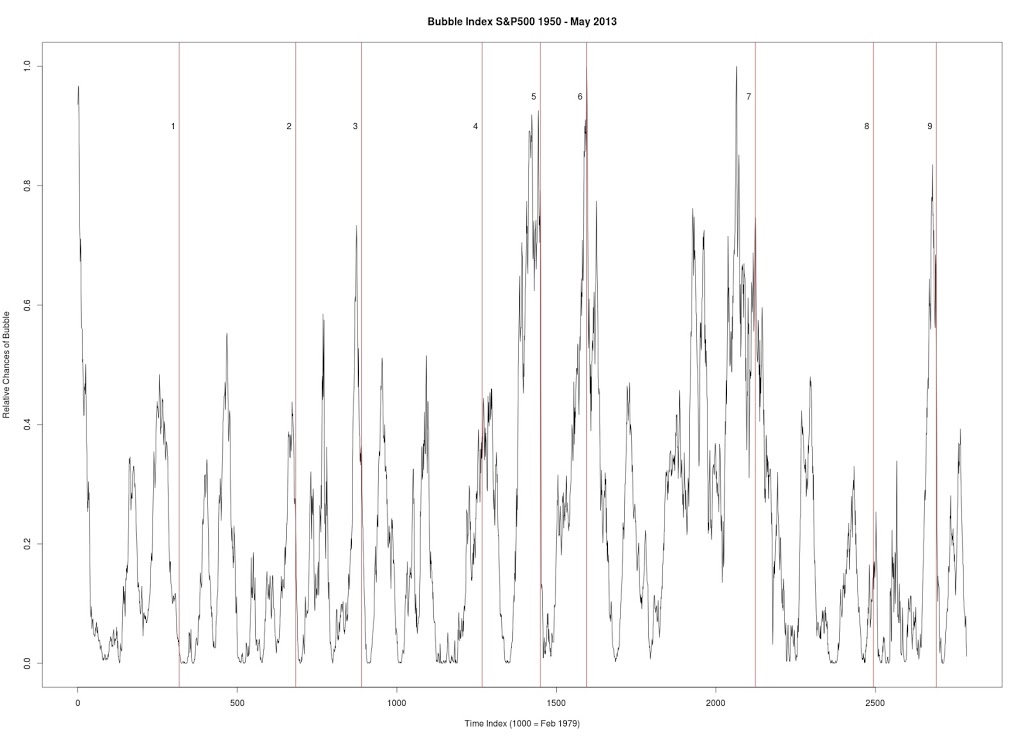
Figure 1

Figure 1 produced with C++ code. S&P 500. Seven year window of data. Every data point is a new week (vs. other graphs where every data point is a change of 4 weeks). Every peak in the market is corresponded by vertical line.
1. January 17, 1966 — followed by a 20.9% drop
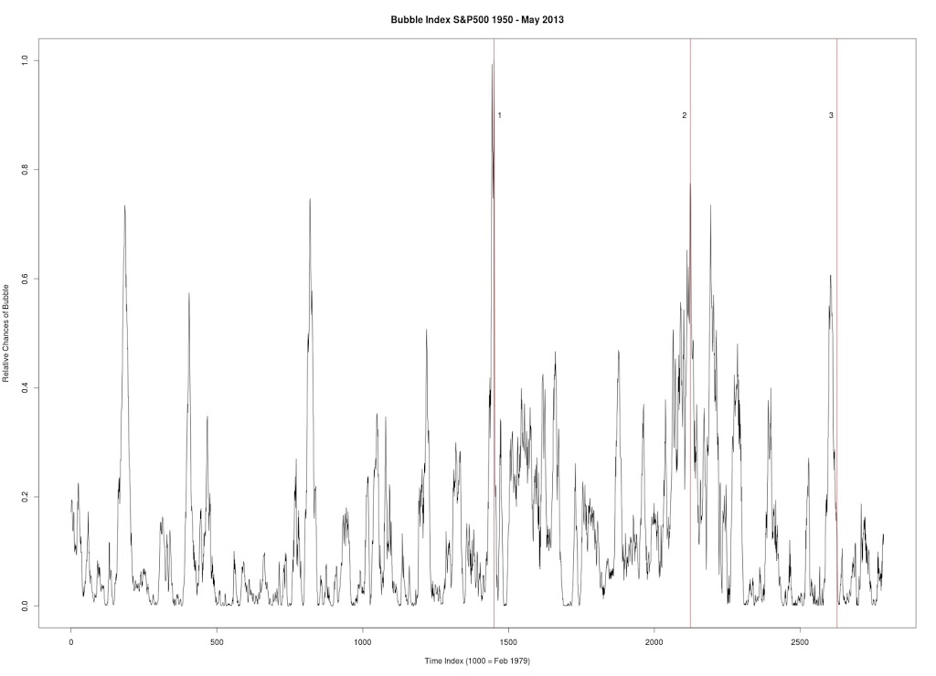
2. January 15, 1973 — followed by a drop in excess of 23%
3. December 27, 1976 — followed by a drop in excess of 14.7%
4. March 26, 1984 — followed by a 11.8% drop
5. Sept. 28, 1987 — followed by a 31.7% drop
6. July 9, 1990 — followed by a 17.4% drop
7. August 28, 2000 — followed by a 36.5% drop
8. October 1, 2007 — followed by a drop in excess of 42%
9. July 18, 2011 — followed by a 16.5% drop

Figure 2

Figure 2 was produced with C++ code. S&P 500. Six year window of data.

1. Sept. 28, 1987 — followed by a 31.7% drop

2. August 28, 2000 — followed by a 36.5% drop

3. April 19, 2010 — followed by a 16% drop
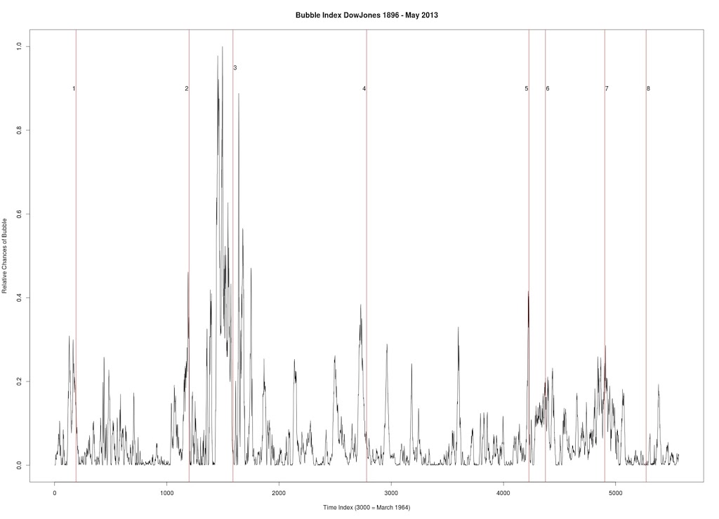
Figure 3

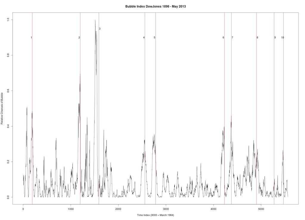
Figure 3 was produced with C++ code. Dow Jones Industrial Average. Six year window of data.
1. December 31, 1909 — followed by a 23% drop
2. October 2, 1929 — followed by a 43% drop
3. March 12, 1937 — followed by a 40% drop
4. January 8, 1960 — followed by a 15.6% drop
5. October 2, 1987 — followed by a 31.7% drop
6. July 27, 1990 — followed by a 17% drop
7. September 8, 2000 — followed by a 36% drop
8. October 12, 2007 — followed by a drop in excess of 42%

Figure 4

Figure 4 was produced with C++ code. Dow Jones Industrial Average. Seven year window of data.
1. December 31, 1909 — followed by a 23% drop
2. October 2, 1929 — followed by a 43% drop
3. March 12, 1937 — followed by a 40% drop
4. September 23, 1955 — followed by a quick 8.7% drop and then recovery
5. January 8, 1960 — followed by a 15.6% drop
6. October 2, 1987 — followed by a 31.7% drop
7. July 27, 1990 — followed by a 17% drop
8. September 8, 2000 — followed by a 36% drop
9. October 12, 2007 — followed by a drop in excess of 42%
10. July 8, 2011 — followed by a 16% drop

Complex System vs. Stochastic Models of Market Returns

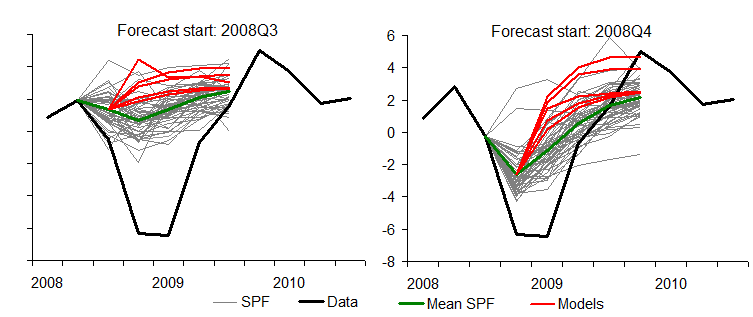
Modelling market returns as independent random variables/martingales is the same as modelling the solar system as a geocentric system with the planets and Sun circling around Earth in epicycles. Predictions of the future are often vastly incorrect in both models. Quite surprisingly, this solar system model survived for thousands of years, despite it being totally incorrect. Then came Tycho Brahe who introduced a modified version of this Ptolemaic system. In Brahe’s model the planets orbit the Sun which orbits the Earth. While this model improved the accuracy of planetary motions, it failed to model reality. Perhaps it could be said that stochastic jump processes are equivalent to Brahe’s model of the solar system. While these jump process do a better job at modelling the returns than simple stochastic processes, they fail to grasp the underlying true model of returns.

Poor Market Forecasting

And as we now know, the true model (for now) of the solar system was introduced by Aristarchus (Copernicus and Kepler helped bring forward this model) and predicts planetary motions with near perfection and represents the actual state of the solar system. I believe that the analogous model for stock returns has been introduced by Didier Sornette, Anders Johanson and others.

These scientists have expounded the idea that market returns are a function of individual agents in a complex system. Just as the human body is a collection of individual cells which make “decisions” based on communications with neighbours through chemical processes, traders make their own decisions based on communication with neighbours. With this perspective the market is a complex system of interacting agents. Thus, returns should be a function of these interactions. Under this complex system model, bubbles and crashes which dot the history of finance (which are not explained fully by independent returns/martingales) are straightforward results. In addition, these models still explain why returns are close to normal “most” of the time.
So, it seems that we need to modify or throw away the old models in favour of these new complex system models. These complex models offer better prediction of the overall market and more fully represent reality.

There is the interesting possibility of this: the stochastic volatility model referred to as the Ornstein-Uhlenbeck process represents the physical process of a “noisy relaxation process.” The Wiener Process represents Brownian motion or motion of a particle through a gas or liquid. So, if we consider the movement of a stock through a virtual container of many stocks (these stocks are the atoms in the Brownian motion) then we need to ask ourselves: What does the price, interest rate, returns, etc. mimic? It is NOT the equations! BUT the physical processes themselves.  Why is an interest rate in a state of disequilibrium in the first place… that it must try to relax? Who put the stock in swarm of human hands all independently moving… It more correctly seems that the traders are following its movement at every second, waiting to grab it when the time if right (thus not independent)?

Can a Stock Market Crash be Avoided? Can the Collapse of Society be Avoided?

The idea in Why Stock Markets Crash is that there exists a critical point which represents the boundary between two regimes. The entire stock market exists as numerous agents whose decisions are not independent.  These agents are in a state of disorder under “normal” trading conditions, thus creating return distributions which are normally distributed. As time progresses the market rises and the agents begin to enter a state bordering disorder and order.  While in this state, the market attitudes of the agents can be abstracted to fractal islands just like the Ising model when close to criticality; in this state, attitudes are able to percolate through various hierarchies and organizations. I have left out many details, but the general concept is that once the market reaches this state, the probability for a crash becomes large; in other words, a crash is the result of instabilities caused by agents reaching a critical state.
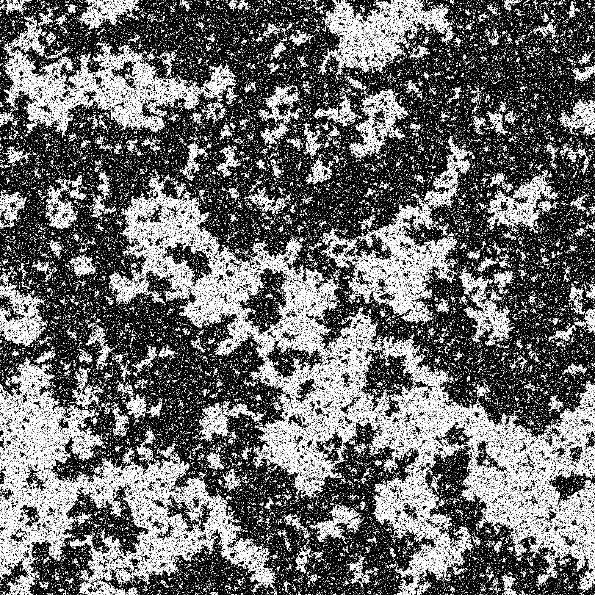
Ising model representing attitudes of agents
My question is this: If market agents realize the instability and expect a crash, will the crash be avoided?
Perhaps there exists a critical proportion of agents who must expect the crash for it to be avoided. If a small number of agents expect the crash, then it will still occur. If more than the critical number of agents expect the crash, it will be avoided. But, if so many agents share the same attitude, doesn’t that make  the market even more unstable? With all this order, there will be opportunities for arbitrage. As attitudes flip-flop and cascade through the system, this arbitrage opportunity will occur again and again; faster and faster; this creates the observed log-periodic oscillations. Eventually, the crash occurs. My conclusion seems to be that a crash can not be avoided.
Figure and Ground
People say that in reality there is no arbitrage. They believe that any pattern which arises will be quickly removed. BUT, isn’t the removal of a pattern a pattern itself? Perhaps similar to Hofstadter’s Figure and Ground? Caution: some Grounds are not themselves Figures. I believe that the ideas presented by Sornette may be the pattern of pattern removal. Perhaps there can be strategies based on the removal of a pattern, which is based on the removal of a different pattern… and so forth.
The potential for crash prevention has applications in societal collapse. My intuition tells me that the two are related. If we can answer the question: Can we prevent the crash of a market? Then we will know the answer to the question: Can we prevent the collapse of a society? To me this seems deeply connected with Isaac Asimov’s Foundation Series. In this series Hari Seldon develops psychohistory (from Wikipedia):

Using the laws of mass action, it can predict the future, but only on a large scale; it is error-prone on a small scale. It works on the principle that the behaviour of a mass of people is predictable if the quantity of this mass is very large (equal to the population of the galaxy, which has a population of quadrillions of humans, inhabiting millions of star systems). The larger the number, the more predictable is the future.

It seems that Asimov is once again ahead of his time!

Page 1 of 2

Become a Friend of GNOME [ GNU Link] kde-user

Powered by WordPress & Theme by Anders Norén